Quick answer
Select your data, open Home > Conditional Formatting and pick a rule. Use Highlight Cells for fixed limits, Top/Bottom for best sellers, Duplicate Values for repeats, data bars or color scales for size, and a formula such as =$C2
Key takeaways
- • Conditional formatting changes a cell's look only when its value meets a condition, and it updates automatically.
- • A formula rule like =$C2
Table of contents 13 sections
- The Example: A Small Wholesaler's Stock Sheet
- What Is Conditional Formatting in Excel?
- Rule 1: Highlight Cells Below a Number
- Rule 2: Color the Whole Row With a Formula
- Rule 3: Flag Stock That Expires Within 30 Days
- How Do You Highlight Duplicates in Excel?
- Rule 5: Add Data Bars to Monthly Sales
- Rule 6: Spot the Top 10 Sellers
- Which Rule Wins When Two Rules Clash?
- Copy, Edit and Clear Rules Safely
- Mistakes That Make Conditional Formatting Go Wrong
- Learn Excel Properly in PSTA's Office Automation Course
- Build This Sheet Tonight
Quick self-test before you read on. Your shop's stock sheet has 300 rows. Can you spot, in under ten seconds, which items are below their reorder level, which medicines expire this month and which product code was typed twice? If the honest answer is no, conditional formatting in Excel is the fix, and it takes about fifteen minutes to set up once.
This post walks through one realistic example of conditional formatting in Excel from start to finish. You will build six rules on a single sheet and learn why each one works. Along the way you will see:
- The built-in rule families and when each one fits
- How to color a whole row with a formula rule
- How to flag duplicates and near-expiry dates automatically
- How rule order decides which color wins
- The mistakes that make formatting slow or wrong
The Example: A Small Wholesaler's Stock Sheet
This is an example business, not a real client. Picture a small medicine and general goods wholesaler in Peshawar. The owner keeps stock in one Excel sheet with these columns:
| Column | Heading | Sample Value |
|---|---|---|
| A | Item code | PK-1042 |
| B | Item name | Paracetamol 500 mg (box) |
| C | Quantity in stock | 8 |
| D | Reorder level | 20 |
| E | Expiry date | 30-Dec-2026 |
| F | Units sold this month | 146 |
Data starts in row 2 and runs to row 300. The owner wants the sheet to answer four questions at a glance: what to reorder, what expires soon, which codes are duplicated and which items sell best. Every rule below answers one of them.
What Is Conditional Formatting in Excel?
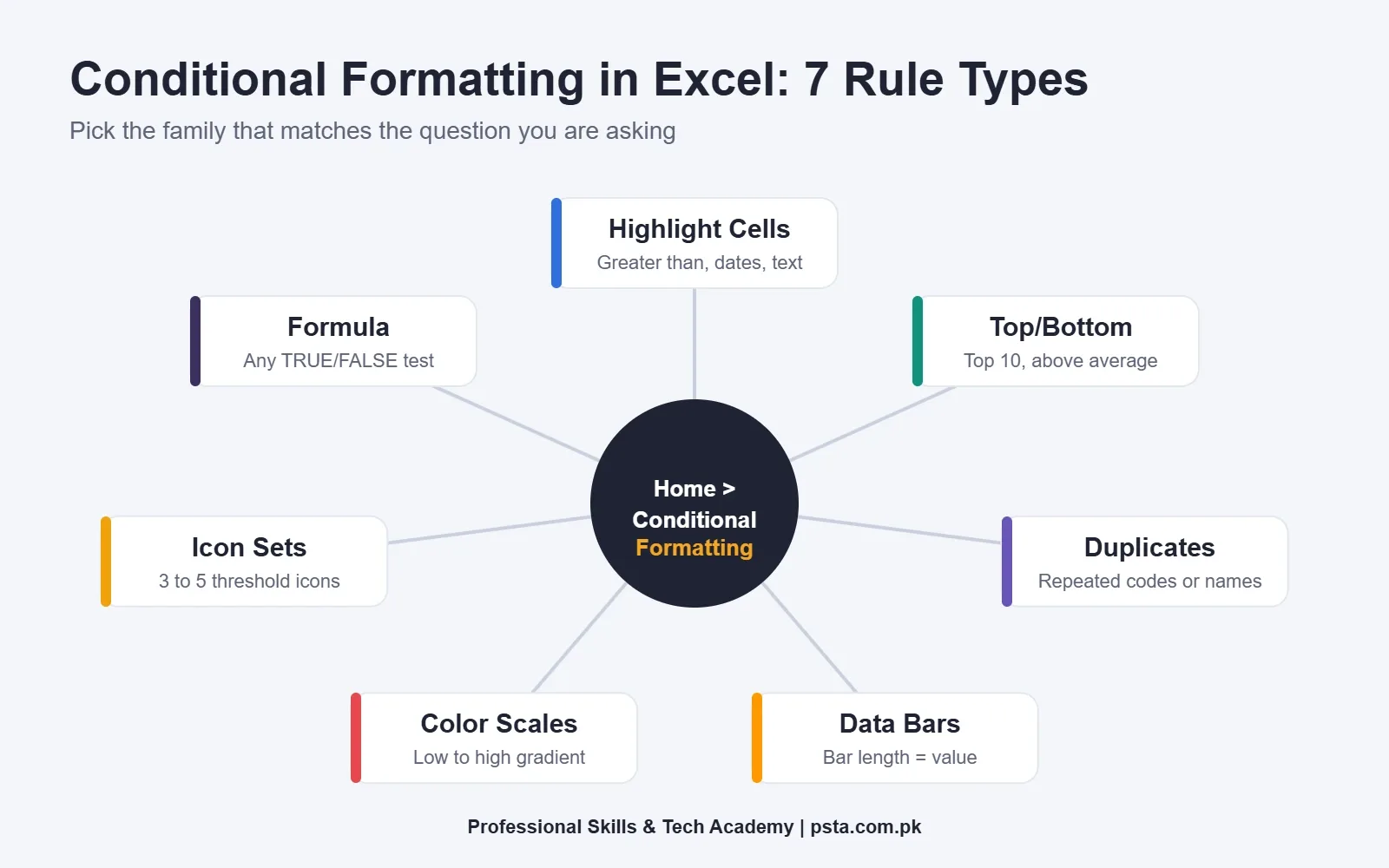
Conditional formatting in Excel changes how a cell looks only when its value meets a condition you set. The formatting updates by itself whenever the data changes, so you never recolor cells by hand. According to Microsoft's conditional formatting guide, the main families are:
- Highlight Cells Rules for comparisons such as greater than, between, text that contains, dates and blanks
- Top/Bottom Rules for the top or bottom items, percentages, or values above and below average
- Duplicate or unique values for spotting repeats
- Data bars, where bar length shows each value's size
- Color scales, two- or three-color gradients from low to high
- Icon sets of three to five icons that sort values by thresholds
- Formula rules for anything the built-in options can't express
All of them live under Home, then Conditional Formatting, in the Styles group. Microsoft's own quick reference card shows the basic flow: select the range, open the menu, pick a rule.
Rule 1: Highlight Cells Below a Number
Start simple, because the easiest conditional formatting in Excel needs no formula at all. Any quantity under 10 should turn red, because the shop is nearly out.
- Select C2:C300.
- Go to Home, Conditional Formatting, Highlight Cells Rules, Less Than.
- Type 10 in the box.
- Choose Light Red Fill with Dark Red Text and click OK.
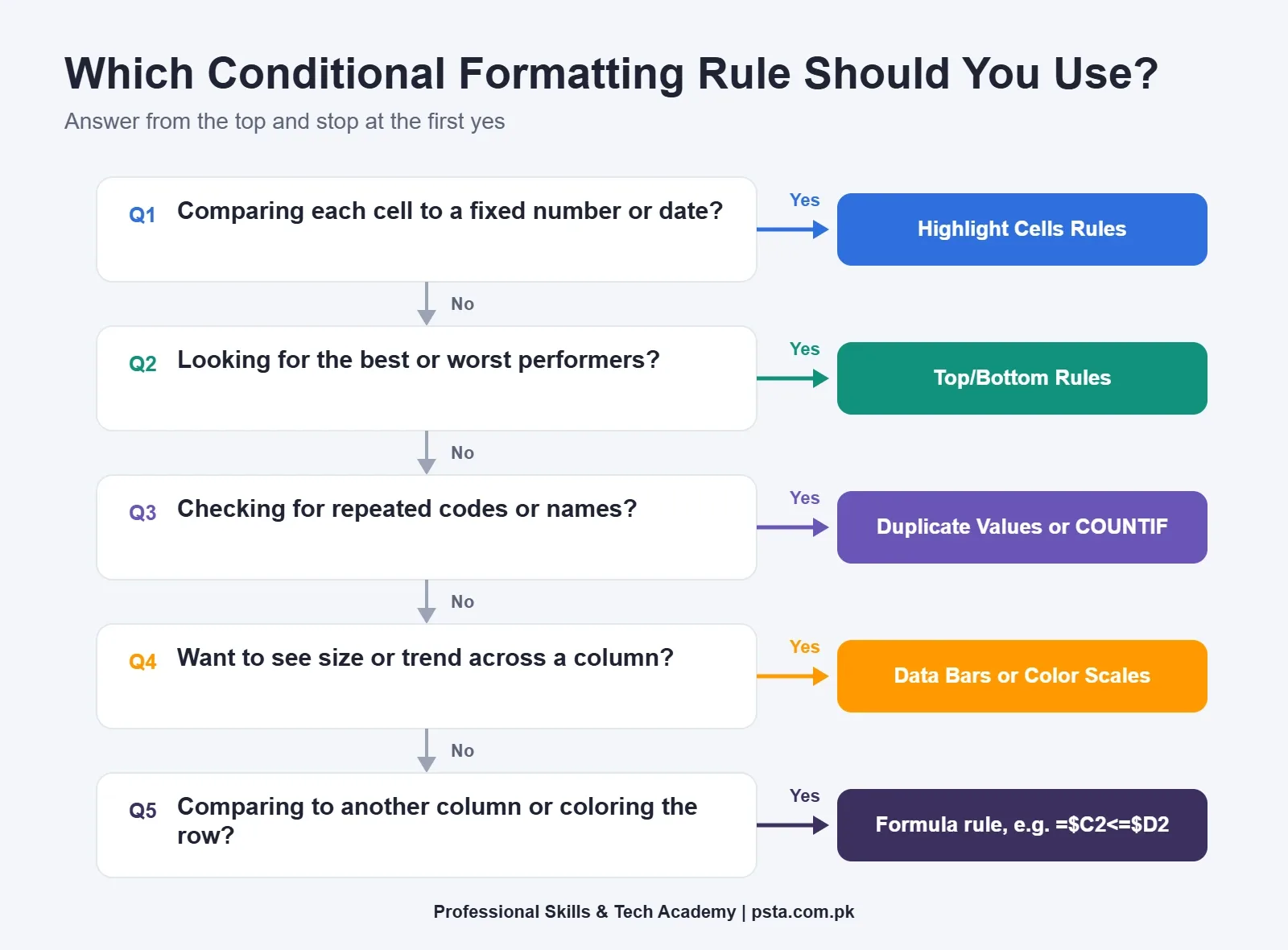
That's the fastest way to highlight cells in Excel. The weakness is the fixed number. Ten boxes might be plenty for a slow item and far too few for paracetamol. Rule 2 fixes that.
Rule 2: Color the Whole Row With a Formula
The owner really wants each row compared with its own reorder level in column D. That needs a conditional formatting formula.
- Select A2:F300, starting from A2 so A2 is the active cell.
- Go to Conditional Formatting, New Rule.
- In the rule type list, pick the option that begins "Use a formula."
- Type
=$C2<=$D2 - Click Format, choose a light orange fill and click OK twice.
Microsoft's page on using a formula to apply conditional formatting shows the same idea: the formula starts with an equal sign, and cells are formatted when its test is met. The dollar signs matter here. $C locks the column, so every cell in the row checks column C. The row number 2 has no dollar sign, so it moves down as Excel checks rows 3, 4, 5 and onward.
Get the dollar signs wrong and you'll see odd stripes of color. If only column A turns orange, or the colors appear one row off, check which cell was active when you typed the formula.
Rule 3: Flag Stock That Expires Within 30 Days
Dates are where these rules save real money. Medicines and packaged food can't sit past their expiry date. Select E2:E300 and add another formula rule:
=AND($E2>=TODAY(),$E2<=TODAY()+30)
Give it a yellow fill. TODAY() returns the current date each time the file recalculates, so the rule stays current without edits. Add a second rule, =$E2<TODAY(), with a dark red fill for anything already expired. A blank expiry cell would count as a very old date, so wrap the test as =AND($E2<>"",$E2<TODAY()) if some rows have no date.
How Do You Highlight Duplicates in Excel?
Select A2:A300 and choose Highlight Cells Rules, Duplicate Values. Excel colors every code that appears more than once. That's usually enough to catch a typing slip where two products share one code.
For more control, use COUNTIF as a formula rule. Microsoft's own formula example uses this pattern, and the COUNTIF function page explains how it counts matches in a range:
=COUNTIF($A$2:$A$300,$A2)>1
Apply it to A2:F300 and the entire duplicated row lights up, which is easier to see than one small cell. The range has dollar signs on both column and row because every check should look at the same list.
Rule 5: Add Data Bars to Monthly Sales
Numbers alone hide patterns. Select F2:F300 and choose Conditional Formatting, Data Bars, then any gradient fill. Each cell now shows a bar whose length matches its sales. Fast movers jump out without sorting.
Data bars in Excel work best on one column of similar numbers. On a column that mixes boxes, cartons and loose units, the bars compare things that aren't comparable, so keep the unit consistent first.
If you prefer a heat-map look, try color scales in Excel instead. A three-color scale shades low sales red, middle values yellow and high sales green. Microsoft notes that the midpoint of a three-color scale defaults to the 50th percentile.
Rule 6: Spot the Top 10 Sellers
Select F2:F300 again and choose Top/Bottom Rules, Top 10 Items. You can change 10 to any number from 1 to 1,000, or use Top 10% instead. Pick a bold green font so it doesn't clash with the data bars already in the column.
Now the sheet answers all four questions, and you haven't recolored a single cell by hand. That is the real payoff of conditional formatting in Excel. Orange rows need reordering, yellow and red dates need attention, duplicate codes stand out, and the best sellers carry both a long bar and green text.
Which Rule Wins When Two Rules Clash?
Open Home, Conditional Formatting, Manage Rules, and set "Show formatting rules for" to This Worksheet. You'll see every rule for that sheet in one list. Microsoft explains that rules are evaluated from top to bottom, and a new rule is added at the top by default.
When two rules don't conflict, both apply. A cell can have an orange fill from one rule and green text from another. When they do conflict, such as two different fill colors, the rule higher in the list wins. Use the Move Up and Move Down arrows to set the order you want.
There's also a Stop If True box beside some rules. Microsoft says it exists mainly for compatibility with older Excel versions, and it isn't available for data bars, color scales or icon sets. For a sheet like this, ordering the rules is enough.
| Order | Rule | Applies To | Format |
|---|---|---|---|
| 1 | =AND($E2<>"",$E2<TODAY()) | E2:E300 | Dark red fill |
| 2 | =AND($E2>=TODAY(),$E2<=TODAY()+30) | E2:E300 | Yellow fill |
| 3 | =COUNTIF($A$2:$A$300,$A2)>1 | A2:F300 | Purple fill |
| 4 | =$C2<=$D2 | A2:F300 | Orange fill |
| 5 | Top 10 Items | F2:F300 | Bold green text |
| 6 | Data bars | F2:F300 | Gradient bar |
Expired stock sits at the top because it is the most urgent. Duplicates come next because they make every other number unreliable.
Copy, Edit and Clear Rules Safely
To reuse rules on next month's sheet, select a formatted cell, click Format Painter and brush it over the new range. Press Esc to stop painting. Microsoft also notes that conditional formatting overrides manual formatting, and removing a rule leaves the manual format underneath.
To start again, go to Conditional Formatting, Clear Rules, and choose either Selected Cells or Entire Sheet. To find every formatted cell on a large sheet, use Go To Special and pick Conditional formats.
The Quick Analysis button, or Ctrl+Q, offers a short menu of formats with a live preview when you select data. It's a handy shortcut for data bars and color scales while you are learning.
Mistakes That Make Conditional Formatting Go Wrong
Most problems with conditional formatting in Excel come from a handful of habits. Check these first when colors look wrong or the file feels slow.
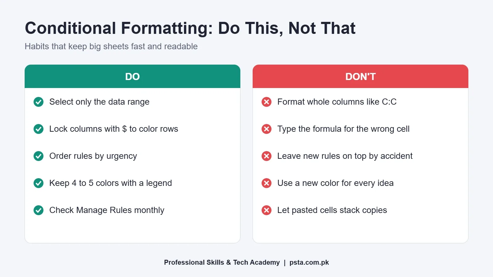
- Selecting whole columns. Rules on C:C check over a million rows. Select only the data range, or format the range as a Table so the rules grow with it.
- Typing the formula for the wrong active cell. The formula must match the top-left cell of your selection.
- Too many colors. More than four or five meanings on one sheet turns into noise. Keep a small legend above the header row.
- Stacking duplicate rules. Copying and pasting cells can multiply rules. Open Manage Rules every few weeks and delete repeats.
- Formulas that return errors. Microsoft notes that a rule whose formula returns an error doesn't format the cell. Wrap risky formulas in IFERROR.
If you're preparing for a computer operator or office assistant test, these rules pair well with the Excel IF function, VLOOKUP vs XLOOKUP and pivot tables in Excel. Our list of Excel interview questions also covers how employers test these skills.
Learn Excel Properly in PSTA's Office Automation Course
Conditional formatting in Excel is one small part of a bigger skill set. Excel work, from tables and formulas to formatting and charts, is one block of the Office Automation course at PSTA (Professional Skills & Tech Academy). The same 12-week beginner program also covers Word, PowerPoint, file management and English and Urdu typing, and one of its projects is a monthly sales sheet with formulas and a chart.
The course page lists the fee as Rs. 12,000, which can be split into two installments. Classes run at the Abbottabad campus, live online for learners elsewhere in Pakistan, or as a hybrid mix, and a new batch opens every month. Compare options on the courses page or apply through admission. If you want a longer route, the one-year DIT diploma includes office skills alongside programming basics.
Build This Sheet Tonight
Reading about conditional formatting in Excel only goes so far. Open Excel, type ten rows of your own stock, fees or expenses, and add Rule 2 and Rule 3 first. Change a few numbers and dates and watch the colors move. Once that works, add the other four rules and check their order in Manage Rules. Stuck on a formula? Send a screenshot on WhatsApp at +92 314 5424399.
Frequently asked questions
How do I apply conditional formatting to an entire row in Excel?
Select the whole data range starting from the first data row, then choose New Rule and the formula-based rule type. Write the formula for the top-left cell and lock the column with a dollar sign, for example =$C2
Why is my conditional formatting not working?
The most common causes are a formula written for the wrong active cell, missing or extra dollar signs, numbers stored as text, or another rule higher in Manage Rules overriding yours. Open Manage Rules, check the Applies To range and the order, and test the formula in a spare cell to see whether it returns TRUE.
Can conditional formatting use another sheet or cell?
Yes, a formula rule can compare a cell with another cell on the same sheet, such as a target in a fixed cell like $H$1. Microsoft notes that rules cannot use external references to a different workbook. If the value lives elsewhere, bring it into the current workbook with a simple link first.
How do I remove conditional formatting from cells?
Select the cells, then go to Home, Conditional Formatting, Clear Rules, Clear Rules from Selected Cells. To remove everything from the sheet, choose Clear Rules from Entire Sheet instead. Manual formatting you applied yourself stays in place, because conditional formatting only sits on top of it.
Does conditional formatting slow down Excel?
It can on large files, especially when rules cover entire columns or the same rule has been copied many times by pasting. Limit each rule to the actual data range, convert the data to a Table if it grows, and clean up repeated rules in Manage Rules. Volatile functions such as TODAY() recalculate often, so use them only where needed.
Is conditional formatting asked in computer operator tests in Pakistan?
Many office and computer operator tests include practical Excel tasks, and formatting data by condition is a common one alongside formulas, sorting and charts. The exact syllabus depends on the employer or testing body, so read the advertised syllabus. Practising rules like the six in this guide prepares you for most practical questions.
What is the difference between data bars and color scales?
Data bars draw a bar inside each cell, so a longer bar means a bigger value and you can compare sizes at a glance. Color scales shade cells with a gradient, such as red for low and green for high, which works like a heat map. Use bars for amounts and scales for spotting high and low zones.
Sources & references
- Use conditional formatting to highlight information in Excel (Microsoft Support) support.microsoft.com
- Use a formula to apply conditional formatting (Microsoft Support) support.office.com
- Quick Reference Guide: Apply conditional formatting (Microsoft) cdn-dynmedia-1.microsoft.com
- COUNTIF function (Microsoft Support) support.microsoft.com
Last reviewed & updated on by Umar Qureshi. Written by the PSTA team in Abbottabad, Pakistan.

Umar Qureshi

Certified Office Automation Course: Master MS Office & Computer Basics
Turn this guide into a career: hands-on training with real projects, online across Pakistan or on-campus in Abbottabad · 12 Weeks.



Comments
No comments yet — ask a question or share your experience.